SIO 210 Talley Lecture 1: Introduction to Ocean Circulation
Lynne Talley, September 26, 1996
Back to SIO 210 index.
Figures
-
Climatological surface temperature and salinity
-
Vertical sections of T, S and O2 in the Atlantic
-
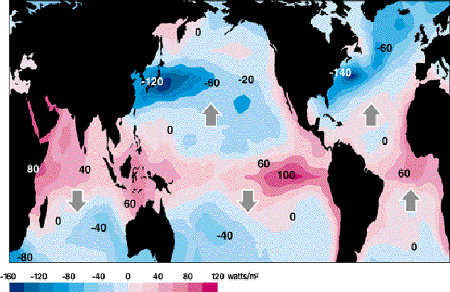
Annual mean net heat flux maps
-
Annual mean net evaporation-precipitation map
-
Example of global wind field
Outline
What is physical oceanography?
What phenomena do physical oceanographers study? (e.g. surface and internal
waves, air-sea exchanges, turbulence and mixing, acoustics, heating
and coooling, wave and wind-induced currents, tides, tsunamis, storm
surges, large-scale waves affected by earth's rotation, large-scale eddies,
general circulation and its changes, coupled ocean-atmosphere dynamics
for weather and climate). Show space and time scales for each.
-
What forces act on the ocean? (e.g. wind [waves, turbulence, large scale
waves, circulation], heating due to the sun and geothermal energy,
cooling, evaporation due to sun and wind, precipitation,
tidal potential [the moon and sun], earthquakes, gravity)
-
How do these forces work on the ocean? Most of them create pressure gradients
which cause water to try to flow from high pressure to low pressure.
The earth's rotation introduces a Coriolis acceleration which induces
flow in the frame of reference of the earth which is to the right of
the motion in the northern hemisphere and to the
left in the southern hemisphere, if the flow persists for about a day
or longer such that it is affected by the rotation. Details for each
follow in Hendershott's lectures.
-
What equations do physical oceanographers use to describe the ocean?
- ma=F (vector form; F = pressure gradient, body forces and dissipation
and a includes time change of velocity, advection and Coriolis
acceleration)
- mass conservation (whatever amount goes into a box must come out)
- equation of state (dependence of density on temperature, salinity
and pressure)
- density changes as a function of heating/cooling and
evaporation/precipitation, and pressure
-
Density of seawater: mass/volume. The density of pure water is about
1000 kg/m3. The density of seawater is about 1020 to 1050 kg/m3, with
the full range mostly due to pressure effects. Ignoring pressure
effects, the range (at sea level pressure) is about 1020 to 1028 kg/m3.
What is the general circulation?
-
Spatial scales: 100s to 1000s of kilmoeters
-
Time scales: small seasonal, interannual to decadal/century changes
in flows which basically retain the same patterns as long as the
land configuration doesn't change and the atmosphere is dominated
by trades and mid-latitude westerlies.
-
Average current speeds: 1-5 cm/sec (horizontal) in the interior
of the ocean, and 100-150 cm/sec (horizontal) in the fastest currents
such as the Gulf Stream and Antarctic Circumpolar Current. Vertical
velocity for the general circulation is on the order of 10-4 cm/sec
and can only be inferred, not measured.
-
Geostrophic balance: in the ma=F equation, the largest terms are the
Coriolis acceleration and the pressure gradient. The time changes,
advection and forcing/dissipation are much smaller.
Description of upper ocean currents.
(zonal = east-west and meridional
= north-south).
Show surface current maps from Tomczak and Godfrey
or Pickard and Emery. Note the great similarities
between the various ocean basins.
Note asymmetry of the gyres: strong western boundary currents and weaker
flow in the interior; weak and shallow eastern boundary currents.
Memorize the names of the western boundary currents.
Subtropical gyres in every
ocean basin (high pressure in the
middle so flow is clockwise in the northern hemisphere and
counterclockwise in the southern hemisphere)
Subpolar gyres in the
two northern hemisphere basins and in the Weddell and Ross Seas (low
pressure in the middle)
Antarctic Circumpolar Current which
is nearly unimpeded flow around Antarctica
Complicated zonal currents in the tropics
Wind forcing: westerlies and trades (see example or Hellerman and
Rosenstein [1983] figures in lecture handout or other wind products)
(Go to wind example.)
Description of large-scale overturning (thermohaline) circulation
Conveyor belt diagram (Broecker, 1991) for the North Atlantic Deep Water cell
gives the sense of the global scale of the overturning, but
is completely missing the Antarctic Bottom Water cell, and is likely
not to be correct in the locations and implied magnitudes and path
of the return flows to the North Atlantic.
Schmitz (1995) diagram: better sense of the complexity of the overturning
pathways. Division of the ocean into 4 layers is sensible (upper
ocean to pycnocline, intermediate layer, deep water layer, bottom
water layer).
Description of temperature and salinity distributions
(Go to surface temperature, salinity figures.)
Surface temperature, showing warmer in tropics and cooler at higher
latitudes. Note large "warm pool" in the western tropical Pacific and
eastern Indian.
Surface salinity, showing highest salinity in the subtropical
evaporation cells and lowest salinity in the precipitation-dominated
subpolar regions.
(Go to vertical section figures.)
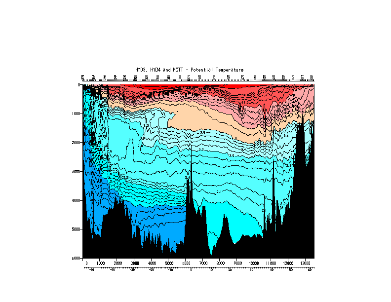
Vertical section of temperature (example at 20W in the Atlantic):
warm at the surface to cold down below. Warm waters reach a bit
deeper in the bowls of the subtropical gyres. Coldest
deep water extending northward from Antarctica. Large rise in
isotherms south of 40S associated with the Antarctic Circumpolar Current.
Temperature inversion layer in the South Atlantic, must be balanced
by salinity since on these large scales true density inversions are never
seen.
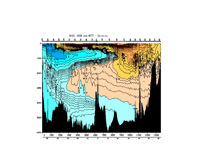
Vertical section of salinity (example at 20W in the Atlantic):
"Four" layers are fairly clear. (1) Saline near-surface layer, with bowls
in the subtropical gyres, (2) intermediate layer with
fresh tongues extending equatorward from the
south (500-1500 meters deep) and north (1200-2200 meters deep)
and a saline layer in the North Atlantic
injected from the Mediterranean (500-2500 meters deep), (3) deep water layer
marked by high salinity extending southward into the South Atlantic,
(4) bottom water layer of lower salinity extending northward from
Antarctica into the North Atlantic.
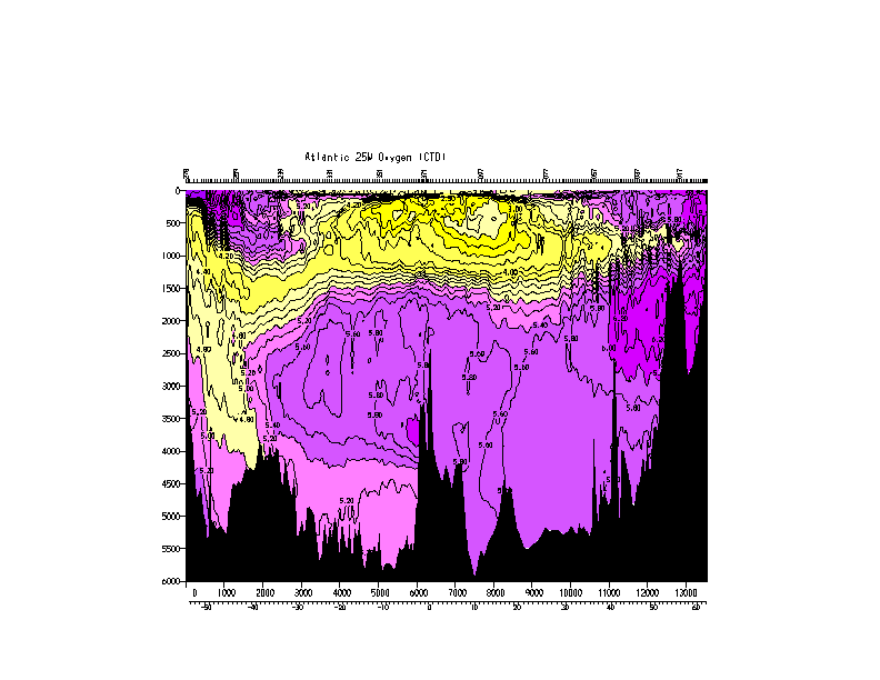
Vertical section of oxygen (example at 20W in the Atlantic):
showing the same four layers as are evident in salinity.
Thermohaline forcing
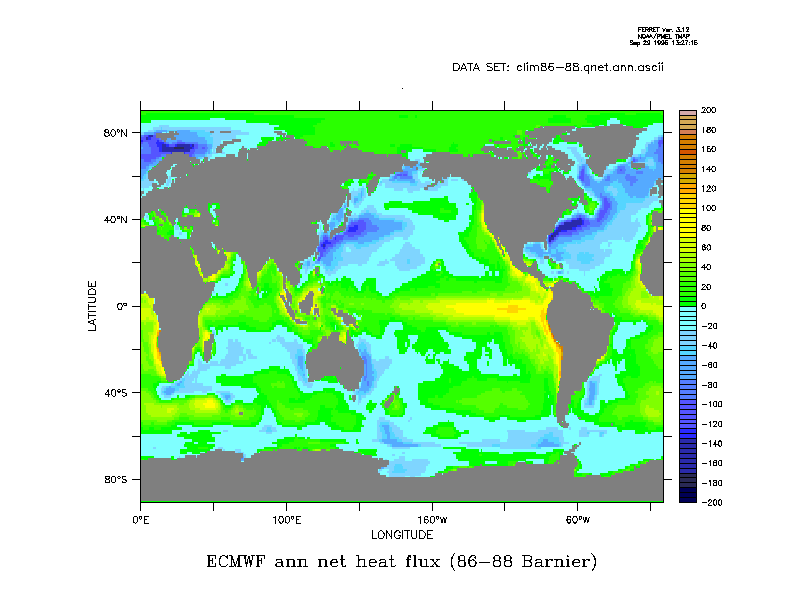
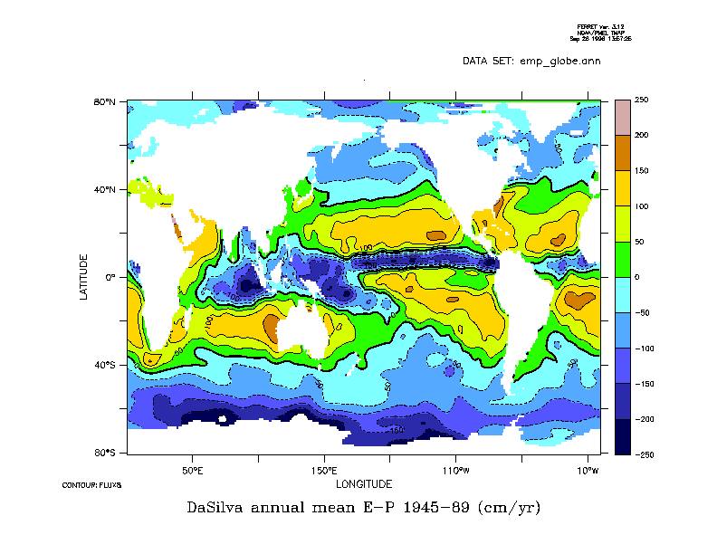
(Go to heat flux and evaporation/precipitation maps.)
The gross aspects of the salinity and temperature distributions, and
the driving force for the slow overturning circulation, are due
to surface heating/cooling and surface evaporation/precipitation/
continental runoff. Maps of heat flux and evaporation - precipitation
are presented. I don't have a net buoyancy flux map for the lecture
notes.
Figures
Annual mean salinity and temperature at 10 meters depth
from the Levitus (1982) climatology. Data for this older
climatology and for a newer one (1994) are available on
nemo.ucsd.edu. To obtain the data, rlogin nemo.ucsd, login
as info, and follow directions for Levitus data.
Atlantic and Indian Oceans:
Temperature
&
Salinity
Pacific Ocean:
Temperature
&
Salinity
Potential temperature, salinity and oxygen (ml/l)
along a
vertical section at 20 to 25W in the Atlantic Ocean.
Potential Temperature,
Salinity,
and
Oxygen
The data were collected in 1988 and 1989 and references are:
Tsuchiya, M., L.D. Talley and M.S. McCartney, 1992. An
eastern Atlantic section from iceland southward across the
equator. Deep-Sea Res., 39, 1885-1917.
Tsuchiya, M., L.D. Talley and M.S. McCartney, 1994. Water-
mass distributions in the western South Atlantic - a section
from South Georgia Island (54S) northward across the
equator. J. Mar. Res., 52, 55-
Annual mean net heat flux (W/m2)
1.
Net surface heat flux from
Hsiung, 1985.
Estimates of global oceanic meridional heat transport. J. Phys. Oceanogr., 15, 1405-1413.
Superimposed on the map are the directions of meridional heat
transport at selected subtropical latitudes, based on direct
oceanic measurements.
2. From Bernard Barnier, using
the ECMWF (European Center for Medium Range Weather
Forecasting) analyses for the years 1986-1988 to compute surface fluxes. The
ECMWF map of heat flux
reproduces a map in the
following publication. Fields were made available by
Bernard Barnier for the map in sam's anonymous ftp site, and
it is placed here for the use of SIO 210 students only as
part of the course. Please use the following reference:
Barnier, B., L. Siefridt and P. Marchesiello, 1994. Thermal
forcing for a global ocean circulation model using a three-
year climatology of ECMWF analyses. J. Marine Systems, 6,
363-380.
Annual mean net evaporation minus precipitation (cm/yr)
Annual mean E-P
in cm/year constructed
from climatology data in DaSilva's online
Atlas of Surface Marine Data.
DaSilva, A. M., C. C. Young and S. Levitus, 1994. Atlas of surface
marine data 1994.
Example of global wind field
from the
FNOC monthly winds, December, 1990.
Taken from the plot package "ferret"'s examples.