MAE 127: Lecture 3
Getting started with Matlab
UCSD computers:
Unix workstations: EBU1-3327, 3329, & 5702
PCs: EBU1-5702 &
EBU2-239
Starting Matlab:
Unix:
> matlab
or
> matlab
-nosplash -nojvm
PC: under the start menu, look for Matlab in the list of available
applications.
Running a tutorial: The
Mathworks has a good tutorial that will help you get started.
http://www.mathworks.com/academia/student_center/tutorials/launchpad.html
If you have used Matlab before, you might check out an alternative
tutorial or help page to refresh your knowledge:
Loading data: If we're
going to analyze data using Matlab, we have to get Matlab to read our
data. The sample data for this lecture come from a 40
year-long computer model of ocean circulation. We'll look at the
surface layer of the tropical Pacific. In general, for this
class, most of the data that you need for
homework will be preformatted for Matlab, so you can just load it by
using the "open" option in the menus or with any of the
following:
load
sample_data.mat
load('sample_data.mat')
The .mat
extension indicates a Matlab binary file. These files can
contain multiple variables that have different dimensions.
From the UCSD PCs, you can access data for this class from the server
ieng9. From the desktop, look for "class resources", and then me127s.pub.
You can use the command who
to list the variables that you have in Matlab's work space. The
command whos will also
show you the size of each variable array.
Plotting:
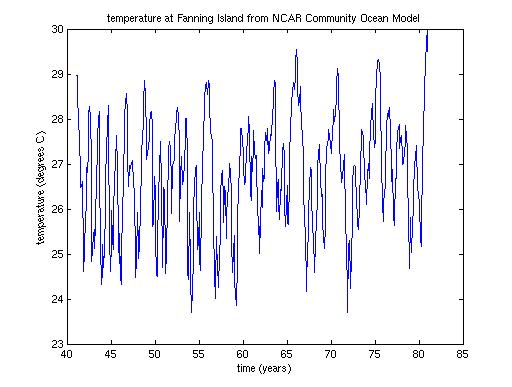
line plots:
plot(time_bound/365,Fan_T)
xlabel('time (years)');
ylabel('temperature (degrees C)')

Alternatively, we could make the same plot from the ASCII data:
plot(DATA2(:,1)/365,DATA2(:,2))
Now what about plotting our big arrays. Plotting all the
data as line plots clearly isn't very useful. Instead we'll want
a way to represent the data in 3-dimensions---latitude, longitude, and
a variable quantity.
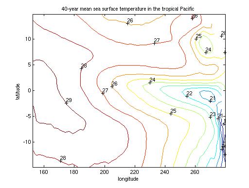
contour plots: Contour
plots show lines of constant property. They work well when
quantities vary smoothly (but aren't so good if you want to plot
discrete quantities.) The following commands produce a contour
plot of temperature at 1 degree intervals, with longitude and latitude
correctly identified, and contours labelled.
c=contour(lon_t,lat_t,T,18:30);
clabel(c)
xlabel('longitude');
ylabel('latitude');
title('40-year mean sea surface
temperature in the tropical Pacific')

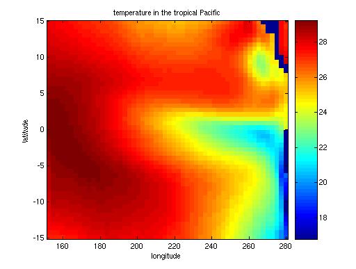
image plots: Shaded
image plots color each grid point according to the value at that point,
so they don't require smoothly varying data values. Matlab
has two functions that handle this: image and imagesc. For many
purposes, imagesc is more
satisfactory, since it automatically scales the color scale to
represent the full range of values in the data.
imagesc(lon_t,lat_t,T); axis xy;
colorbar;
xlabel('longitude');
ylabel('latitude');
title('salinity in the tropical
Pacific')

The Matlab image functions order arrays like mathematical matrices with
coordinate (1,1) in the upper left corner. Data tend to start
with the smallest latitude and longitude values, which should be mapped
in the lower left corner. To make your Matlab image plot look
correct, you can use axis xy,
as above, or you can flip the matrix top-to-bottom: imagesc(lon_t,lat_t,flipud(T));
saving figures: Finally,
Matlab gives you several ways to save figures. To save a plot
that you want to edit more carefully, use the "Save" option under the
Figure window "File" heading. This will give you a file with a
.fig ending that will allow you to pick up where you left off editing a
Matlab figure, but it won't give you a generic format that you can
print out. Do not send me .fig files.
You can also use the "Save As" option under the "File" heading to save
your work as a jpg, gif, tiff, postscript (ps), encapsulated postscript
(eps), or a number of other formats which are convenient for posting to
the web, including in other documents, or e-mailing to your professor.
If you want to save a file to print, you can use the print option to
send it straight to the printer or to write it into a file as
postscript.
Computing a histogram: Sometimes
we want to plot a histogram of all the data values acquired in a
particular region or at a particular point in time. For
example, it might not make sense to plot heights of everyone in the
classroom as a function of anything. (What would you use?
arrival time? geographic coordinate in the classroom?
age? shoe size?) Matlab makes histograms automatically.
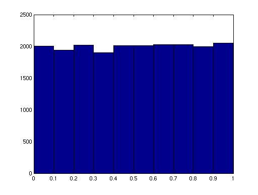
Let's define a
set of random numbers x:
x=rand(20000,1);
hist(x)
If we don't like the number of bins that Matlab has used, we can
specify some formating details:
hist(x,30)
uses 30 bins.
hist(x,0.05:.1:.95) uses
bins
centered at 0.05, 0.15, 0.25, ... 0.95.

Computing means and standard
deviations: Matlab has a number of built in functions to
compute many basic statistical quantities. Here are a few:
- mean(A) computes the
average of each column of the matrix A.
- mean(A'), computes
the average of each row of the matrix A. Here we use the ' to tell Matlab to take the
transpose of A. But
watch out if A contains
complex numbers. Following standard mathematical notation, the
transpose of A has
complex conjugates. Thus 1+2i
in A becomes 1-2i in A'.
- mean(A,1) is the
same as mean(A).
The 1 says to compute the average over the first dimension in A.
- mean(A,2) is a lot
like mean(A'), though it
doesn't rotate the results, and it avoids problems with complex
conjugates.
- std(A) or std(A,0,1) computes the
standard deviation of each column of matrix A.
- std(A') or std(A,0,2) will provide
standard deviations for the rows of A.
- Sometimes missing data points are filled with not-a-number (or
NaN). The mean of a data set that contains a NaN is
NaN. The matlab function nanmean will ignore NaN values
when it computes the mean.
Automating a procedure: What
if you want to repeat the same calculation with a series of different
parameters? Here is one strategy:
run a for loop: loop through a series of
variables, performing a calculation for each one.
for
i=3:8
array=reshape(A(:,i),nlat,nlon);
figure(i-2)
imagesc(array,lat,lon)
end
Making an M-file:
Programs that run in Matlab are identifiable because they end in
.m. An M-file consists of a series of instructions that you want
Matlab to execute. They can be set up as simple sets of
instructions:
x=rand(10,1);
mean(x)
or as functions:
function
z=test_function(x)
% This M-file, test_function.m, computes the column mean of input data
x.
z=mean(x);
end
This one would be executed by typing test_function(x). Matlab
programs don't need to be compiled, so they aren't always very
efficient, but they can contain some fairly sophisticated programming
concepts.
How do you create a Matlab .m file? New versions of Matlab have
an option under "File" to let you open a new M-file to edit. In
any version, you can also use a plain text editor to create your Matlab
program.
Finding help: To find more details on any matlab
function, you can always type help and the name of the function.
Matlab's web site also offers extensive guidance: http://www.mathworks.com/support/product/product.html?product=ML
