MAE 127: lecture 6

MAE 127: Lecture 6

More on Matlab

The goals for this computer session are to help you learn some additional Matlab tricks that will help you out with real data analysis, including providing guidance for the problems that you encounter in this class.

Data formats. Loading other data: Last time we loaded Matlab binary files (with the suffix .mat) using:

load sample_data.mat
load('sample_data.mat')
But not all data is in Matlab binary format.

For plain text (or ASCII) files, Matlab also loads data fairly automatically:

load sample_data.ascii
DATA=load('sample_data.ascii'); and DATA2=load('lecture3.timeseries');
DATA=load('-ascii','sample_data.ascii');

What about Microsoft Word files or Excel spreadsheets? These have binary data formating that Matlab is not designed to read. Save them as plain text, and load them as ASCII files.

Other types of binary data files that you might encounter include:

netcdf: This is a self-documenting file format that is commonly used for geophysical data. The files are easy to read into Matlab if you install the netcdf libraries on your system and the netcdf toolbox. We'll steer clear of these for this class.
hdf: This is another self-documenting file format, though it comes in different flavors. NASA decided on one version of hdf as a standard for satellite data collected by the Earth Observation Satellites. Matlab has an hdf interface that might now work for NASA hdf files.
raw binary: These might include output files from computer simulations, or data files archived in a compact format. Binary files are often classed as "big-endian" or "little-endian". The terminology is an allusion to Jonathan Swift's Gulliver's Travels, and refers to the arbitrary standards used to write binary data on different computer systems. In general, PCs use one format; high end unix workstations often use the other. To read these files in Matlab, you can do the following:

fid=fopen('file.bin','r'); or one of the following if the file was written on a different type of computer: fid=fopen('file.bin','r','l'); or fid=fopen('file.bin','r','b');
a=fread(fid,'float'); to read the entire file. Check the fread documentation to find out how to read part of a file, or to read files that have some floating point numbers and some integers.
fclose(fid); to clean up and avoid hogging all the input/output channels.

Clearing data: Sometimes you want to clear data out of memory. To clear everything and start afresh use:

clear

To clear one or two variables:

clear x y

Representing a matrix: Matlab is really designed to work with matrices, so it very naturally stores data in two dimensional arrays, and will also use arrays of arbitrary dimension size. If you read in your data as an ASCII file, you might end up with a big data array containing latitude in the first column, longitude in the next, temperature and the third, and so forth sort of like this:

DATA = [latitudes longitudes salinity temperature velocity(east/west) velocity(north/south) velocity(vertical)];

That's perfect for some purposes, but if your original data came from a two dimensional grid---perhaps they represent sea surface temperature in the tropical Pacific---then we might want to format the data some other way. Here's one way to handle it:

SST=reshape(DATA(:,4),nlat,nlon);

will create an nlat by nlon array containing the temperature data from column 4 of A.

Looking at the data:

To look at the contents of a variable, you can always type its name. You can also specify specific elements of an array. For example:

>> T(1:5,1:5)

ans =

   27.2218   27.2415   27.2729   27.3757   27.4669
   27.4352   27.4828   27.4918   27.5867   27.6677
   27.6014   27.6939   27.6883   27.7699   27.8425
   27.7381   27.8820   27.8640   27.9348   27.9986
   27.8452   28.0494   28.0191   28.0774   28.1343

This is useful for some purposes, but we can't tell much about our temperature data by looking at it this way.

In Matlab, the first index corresponds to the row, and the second to the column. So the second row is:
>> T(2,1:5)

ans =

   27.4352   27.4828   27.4918   27.5867   27.6677
And the second column is:
>> T(1:5,2)

ans =

   27.2415
   27.4828
   27.6939
   27.8820
   28.0494

On the otherhand, we can treat a two dimensional array as a vector by using a single index. Thus:
>> T(1:5)

ans =

   27.2218   27.4352   27.6014   27.7381   27.8452
This provides the first 5 elements in column 1, i.e. T(1:5,1).

More on plotting:

The Matlab image functions order arrays like mathematical matrices with coordinate (1,1) in the upper left corner. Data tend to start with the smallest latitude and longitude values, which should be mapped in the lower left corner. To make your Matlab image plot look correct, you can use axis xy, as above, or you can flip the matrix top-to-bottom: imagesc(lon_t,lat_t,flipud(T));

controlling details of your plots: As you work with more data, you may want to control the types of lines you use for plots, line color, or even the range of colors in an image plot. Lots of information is available from the help files. Here are a few pointers.

For simple line plots, lines are ordered blue-green-red-cyan-magenta-yellow-black, but you can override this by specifying a single letter color code (e.g. plot(DATA2(:,1),DATA2(:,2),'r') for a red line.)   You can also specify a line type as solid ('-'), dashed ('--'), dotted (':'), or dash-dotted ('-.').

To plot data as points (particularly useful when your data aren't ordered sequentially), make a scatter plot by specifying a symbol only:

plot(DATA2(:,1),DATA2(:,2),'o')

to plot circles.

If you start creating a plot and want to keep adding to it, use the hold on command to prevent Matlab from erasing the first plot when you add a new line and the hold off command to revert to normal mode. The command clf will clear everything out of a figure window to let you start again.

colormaps: In Matlab, the default colormap for contour and image plots is a blue to red spectrum, but you can override this. To change the colormap used for contour or image plots, you can specify a different basic color map by typing, for example, colormap(cool). Other colormaps include hsv, prism, gray, hot, cool, copper, flag, pink, bone, and jet (the default).

Sometimes, you want to make sure that NaNs don't end up shaded the same color as useful data points, so you can force values at the end of your range to be white or black, for example.

cmap2=[[1 1 1]; colormap; [1 1 1]];
colormap(cmap2);

You might have to fix the limits of your colors to keep real data from also being whited out. To get black where you had no data, you'd use [0 0 0].

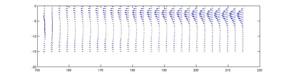
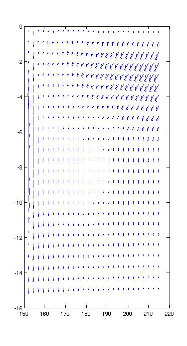
Plotting vector quantities: Velocity vectors can be a little subtle. The Matlab function quiver will plot vector quantities. So:

quiver(lon_t,lat_t,U,V)

plots a map of vector velocities. The results are a little deceptive. If you change the aspect ratio of the plot, the vectors appear to change direction, so the on screen vectors aren't telling you the precise direction of the current.

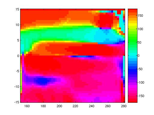
We can also compute the angular direction of the current and plot that as an image:

theta=atan2(V,U)*180/(pi);

Here we use atan2 rather than atan, because we want our angles to go from 0 to 360 degrees. Since 0 and 360 degrees are equivalent, it's good to choose a colorscale where the colors are 0 and 360 are nearly the same. The clrscl.m function (written by an SIO researcher) provides one way to fix a colorscale appropriately. Compare:

imagesc(lon_t,lat_t,theta); axis xy; colorbar

with

colormap(clrscl('rmbcgyr',36))
imagesc(lon_t,lat_t,theta); axis xy; colorbar

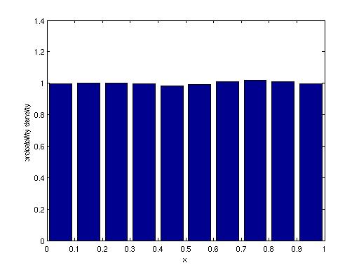
Probability density functions and histograms: We looked at the hist function last week. How do you convert a histogram into a probability density function?

x=rand(20000,1);
[a,b]=hist(x,0.05:.1:.95);

Now we can make a bar plot, typing

bar(b,a)

We can also modify the bar plot to give us what we need for a pdf:

bar(b,a/sum(a)/.1); % where 0.1 is the interval dx
xlabel('x'); ylabel('probability density')

You can get rid of the space between the bars by supplying a width parameter to bar:

bar(b,a/sum(a)/.1,1);

In contrast to this procedure, the Matlab function pdf.m returns the functional form of a specified probability density function.

Logic: Sometimes we want to test for a particular condition. In Matlab, conditional statements can use if, while, or switch. These test whether an expression is true or false. Expressions test the relationship between two quantities. The help page for relop explains everything. Here are some examples.

To test whether T is less than 999, use (T<999).
To test whether T is equal to 999, use (T==999).
To test whether T is not equal to 999, use (T~=999).
To test whether T and S are both not equal to 999, use (T~=999 & S~=999).
To test whether T or S is equal to 999, use (T==999 | S == 999).
To test whether T is NaN, use (isnan(T)).

Automating a procedure: Last week we looked at for loops. Here are some other ways to make a calculation loop:

run a while loop: if you prefer to set a logical test to figure out how many times to run your loop, you can use a while loop. For the example above, you could say:

i=3;
while i<size(A,2)
array=reshape(A(:,i),nlat,nlon);
figure(i-2)
imagesc(array,lat,lon)
i=i+1;
end

use Matlab's vectorization capabilities: For many purposes, Matlab will naturally loop through a whole set of variables without requiring a loop. For example, if you wanted to compute the mean and standard deviation of each column in A, you might be tempted to create a loop:

for i=3:8
m(i-2)=mean(A(:,i));
s(i-2)=std(A(:,i));
end

But instead you could say:

m=mean(A(:,3:8)); s=std(A(:,3:8));

This second option not only requires less code, but it is also computationally faster.