SIO 221C: Color Maps and Images
Images: The Matlab image
functions order arrays like mathematical matrices with
coordinate (1,1) in the upper left corner. Data tend to start
with the smallest latitude and longitude values, which should be mapped
in the lower left corner. To make your Matlab image plot look
correct, you can use axis xy,
or you can flip the matrix top-to-bottom: imagesc(lon_t,lat_t,flipud(T));
Colormaps: In Matlab,
the default colormap for contour and image plots is a blue
to red spectrum, but you can override this. To change the
colormap used for contour or image plots, you can specify a different
basic color map by typing, for example, colormap(cool). Other
colormaps include hsv, prism, gray, hot, cool, copper, flag, pink,
bone, and jet (the default).
Sometimes, you want to make sure that NaNs don't end up shaded the same
color as useful data points, so you can force values at the end of your
range to be white or black, for example.
cmap2=[[1
1 1]; colormap; [1 1
1]];
colormap(cmap2);
You might have to fix the limits of your colors to keep real data from
also being whited out. To get black where you had no data, you'd
use [0 0 0].
Colormaps and color blindness:
About 8% of men and 0.5% of women have color-impaired vision.
Often this means that red and green are difficult to distinguish, which
means that the Matlab default 'jet' colormap can be difficult to
interpret. Better choices are single color schemes (such as
Matlab's 'hot') that increase in intensity, or diverging schemes that
extend from blue to red. For a reprint of the recent EOS article,
comments, and reply see: http://geography.uoregon.edu/datagraphics/EOS/index.htm
For general information
see:
http://geography.uoregon.edu/datagraphics/index.htm
or for tools to check your graphics:
http://www.vischeck.com/vischeck/
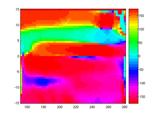
Colormaps and the branch cut:
We can also compute the angular direction of the current and plot that
as an image:
theta=atan2(V,U)*180/(pi);
Here we use atan2 rather than atan, because we want our angles
to go from 0 to 360 degrees.
Since 0 and 360 degrees are equivalent, it's good to choose a
colorscale where the colors are 0 and 360 are nearly the same.
The clrscl.m function (written by Matt Dzieciuch of IGPP)
provides one way to fix a colorscale
appropriately. Compare:
imagesc(lon_t,lat_t,theta);
axis xy; colorbar
with
colormap(clrscl('rmbcgyr',36))
imagesc(lon_t,lat_t,theta); axis
xy; colorbar