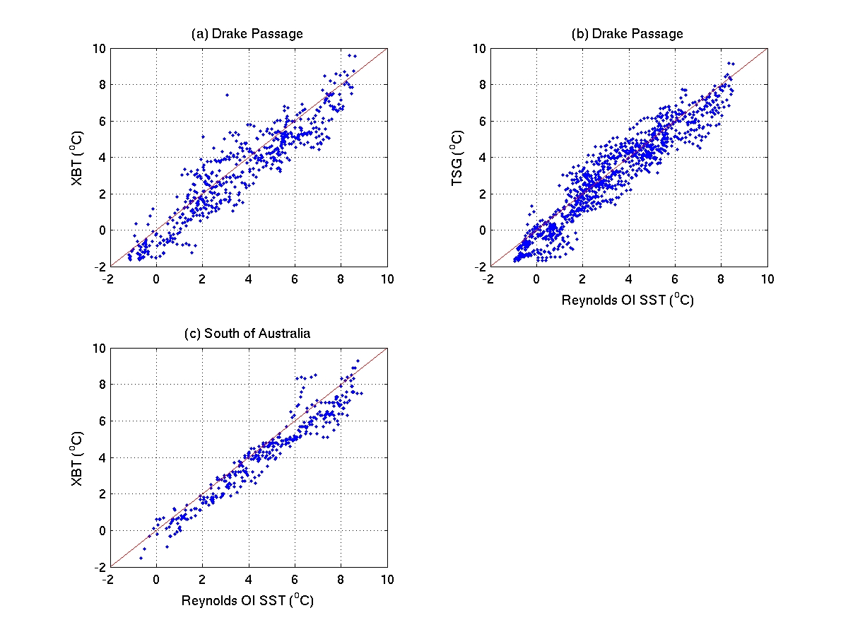
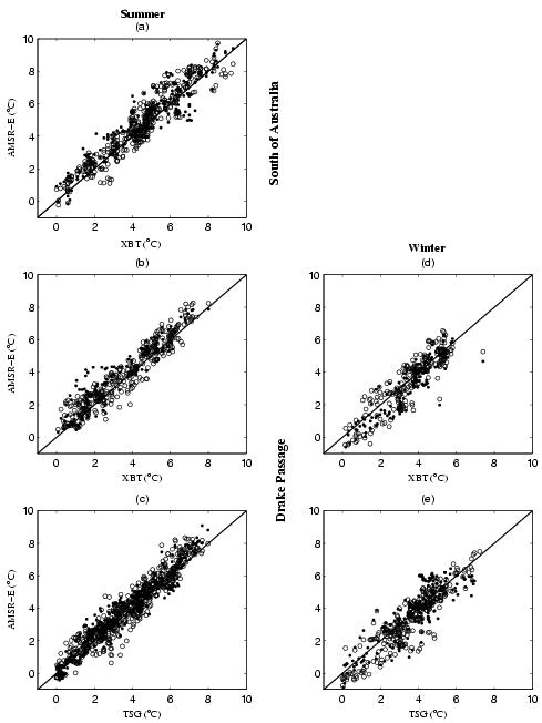
Figure 1 Scatter plot of the XBT/TSG against AMSR-E ascending (dot) and descending (circle) measurements.
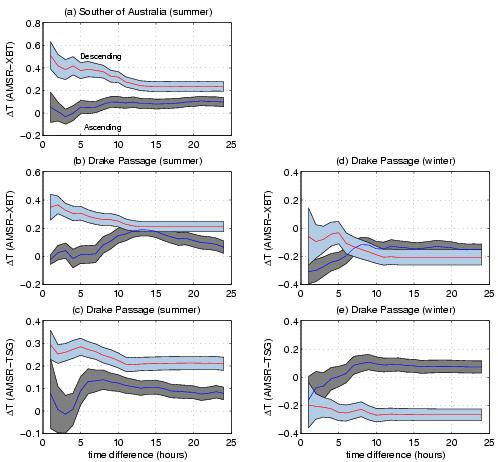
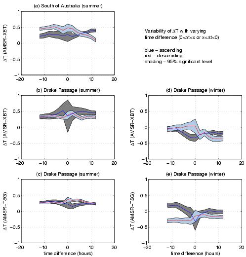
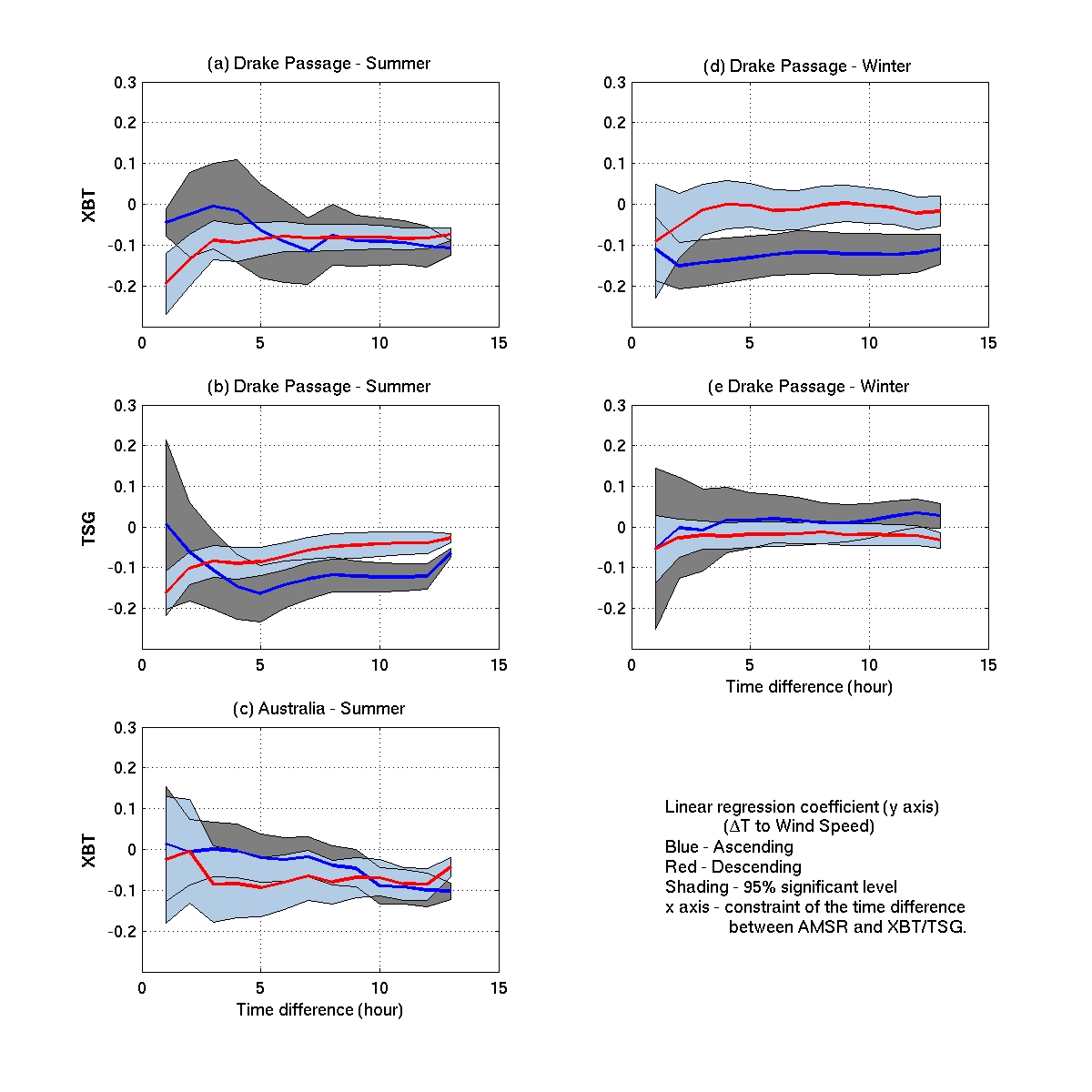
Figure A shows the changes in the mean temperature difference with changes of the constraint on time difference (|dt|<=x). Here is the figure for the time difference going forward and backward Figure B.
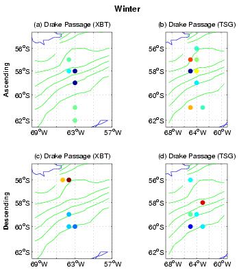
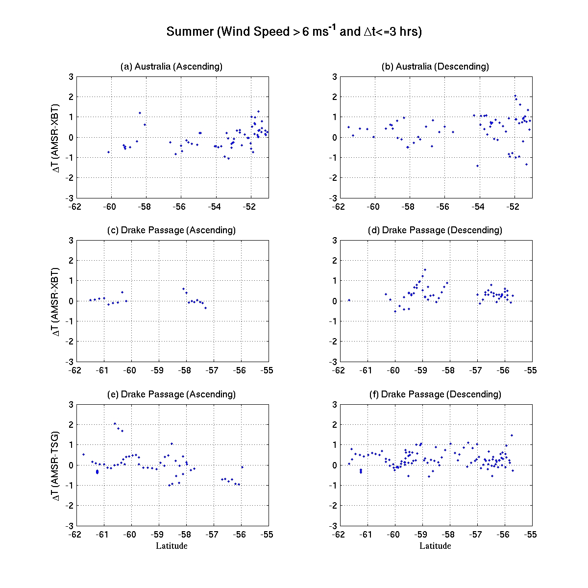
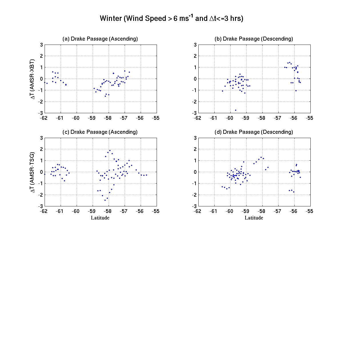
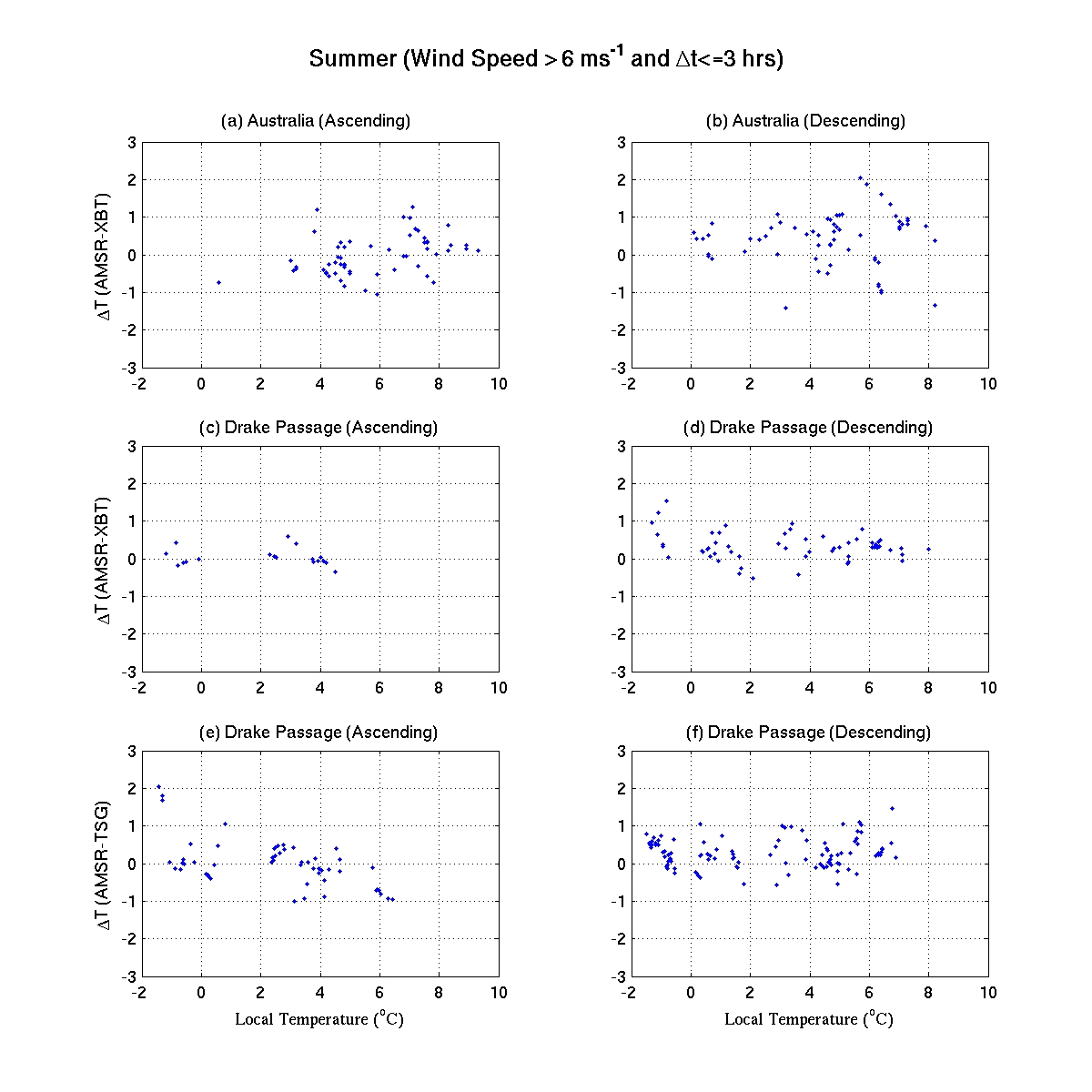
Spatial distribution of the temperature difference for summer and winter after removing low wind speed (6m/s) data and limiting the time difference within 3 hours.
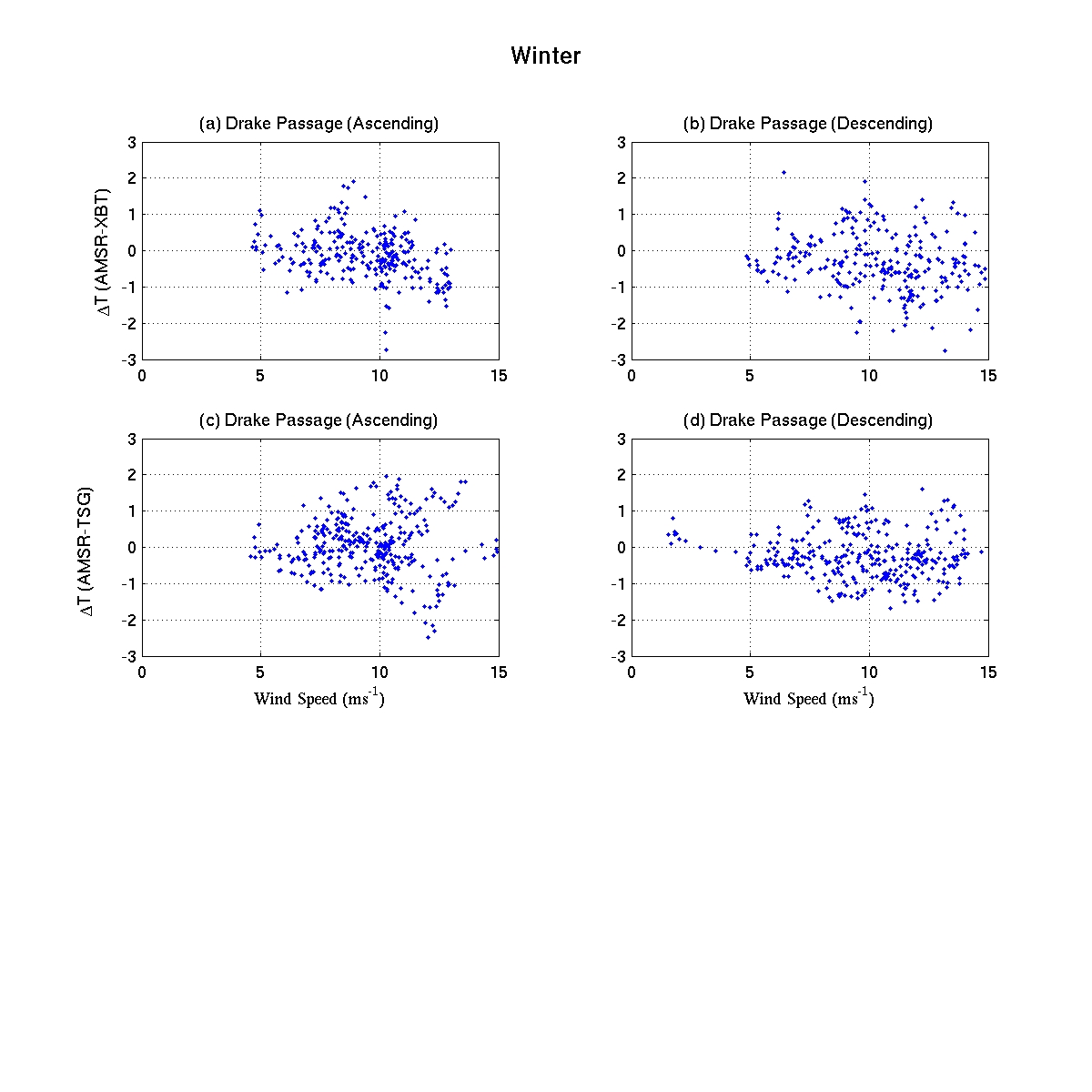
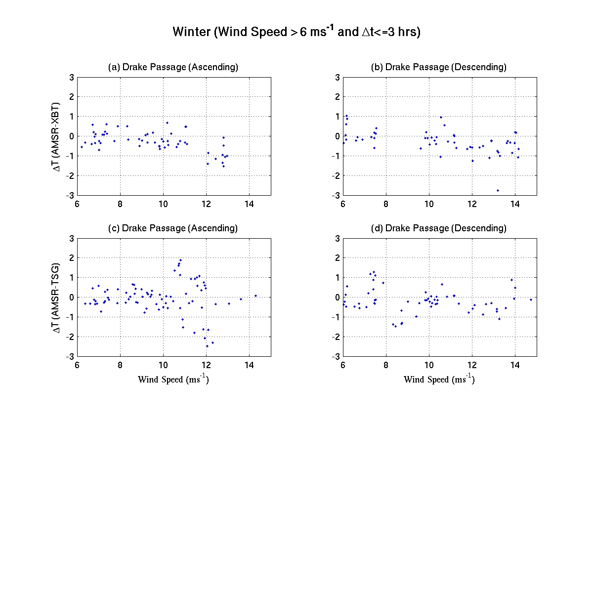
Figure 2 Temperature difference (AMSR-XBT/TSG) against wind speed from AMSR-E for summer (October - March). Figure 3 is for winter. All indicate the decrease of the temperature difference with increase wind speed. Similar to Figure 2 and 3, Figure 4 and Figure 5 are the scatter plots after removing the data with wind speed less than 6 m/s and constrained the XBT data within 3 hours of the observations time of AMSR-E. We can still see the decrease of the temperature difference with increase wind speed.
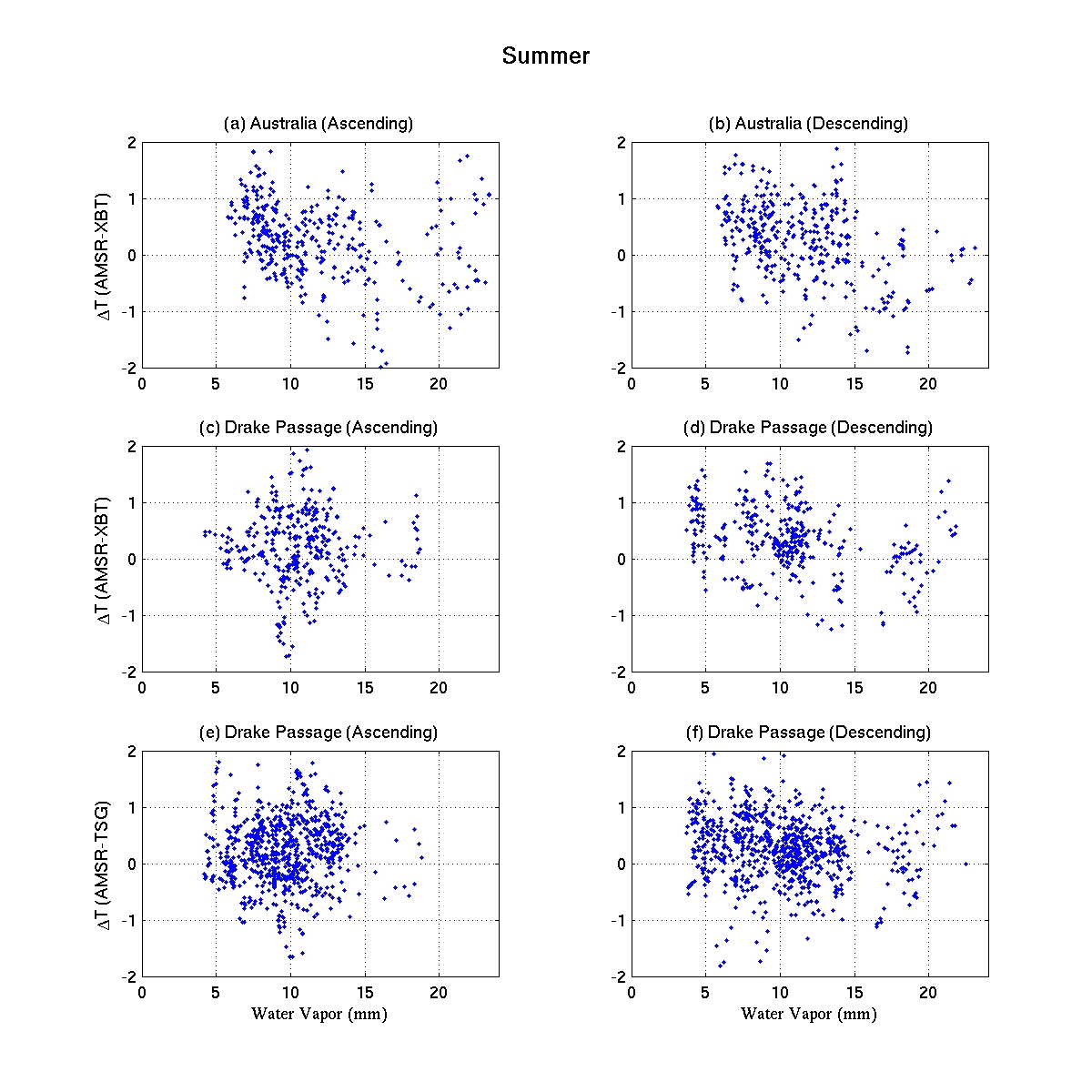
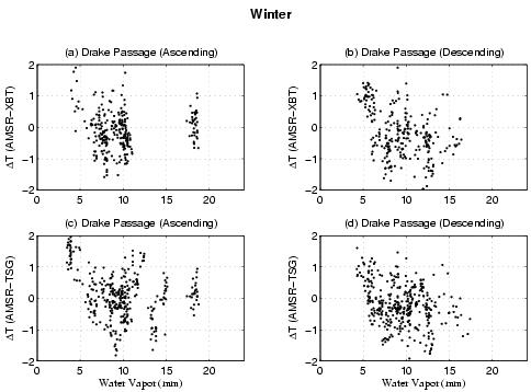
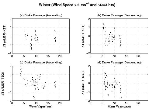
Figure 6 and Figure 7 show the temperature difference against water vapor from AMSR-E for summer and winter, respectively. Temperature difference decrease with increase of water vapor, which are also shown from the plots after removing low wind speed data and constrain the data within 3 hours Figure 8 and Figure 9
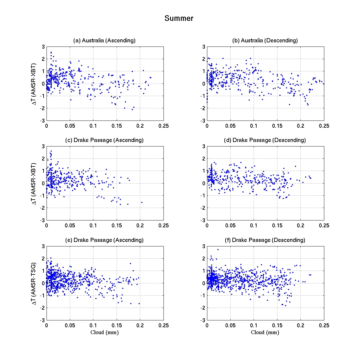
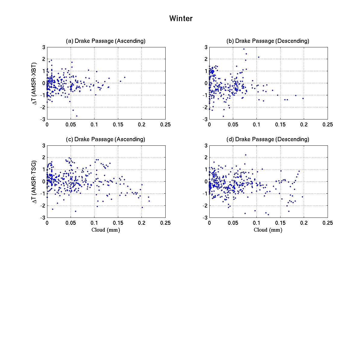
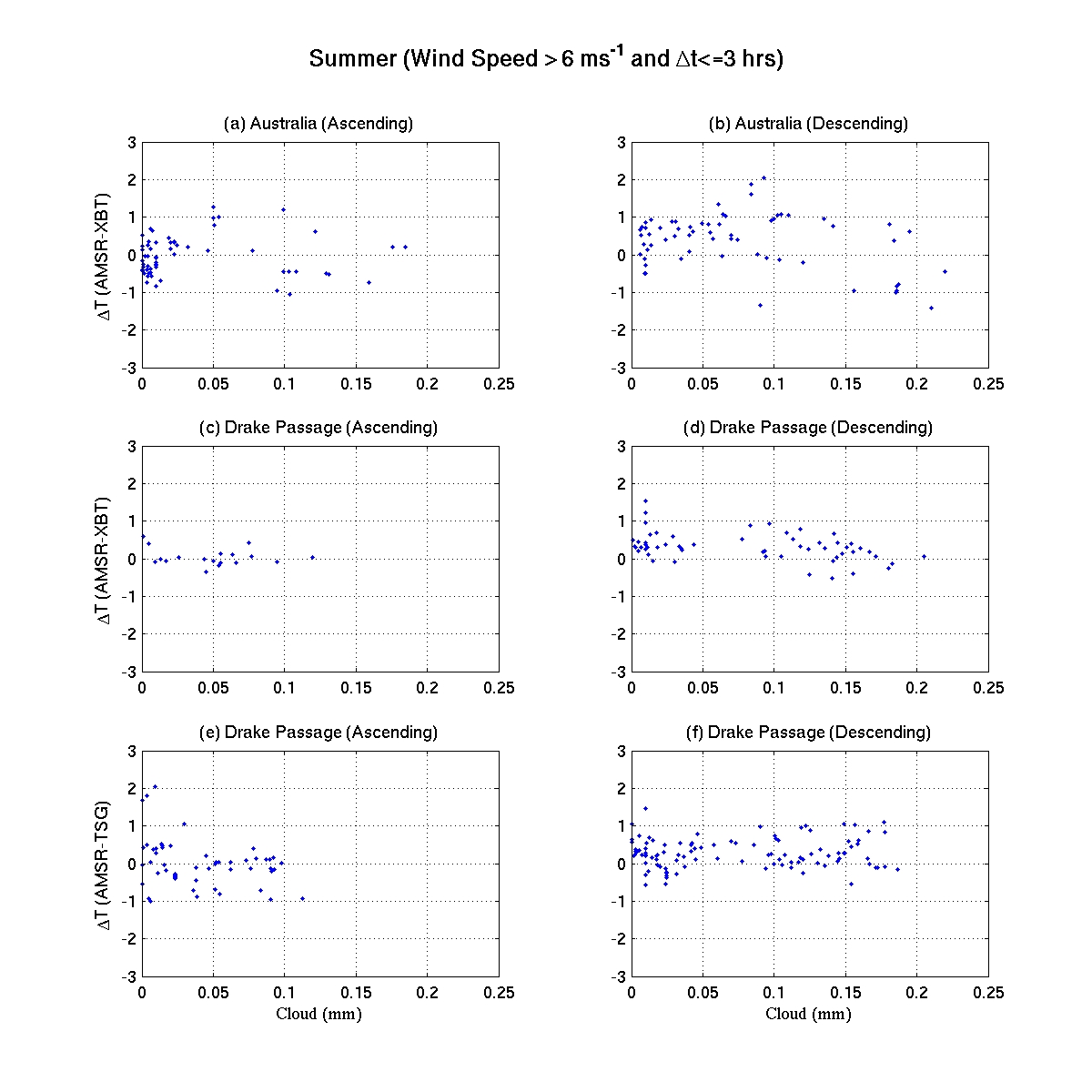
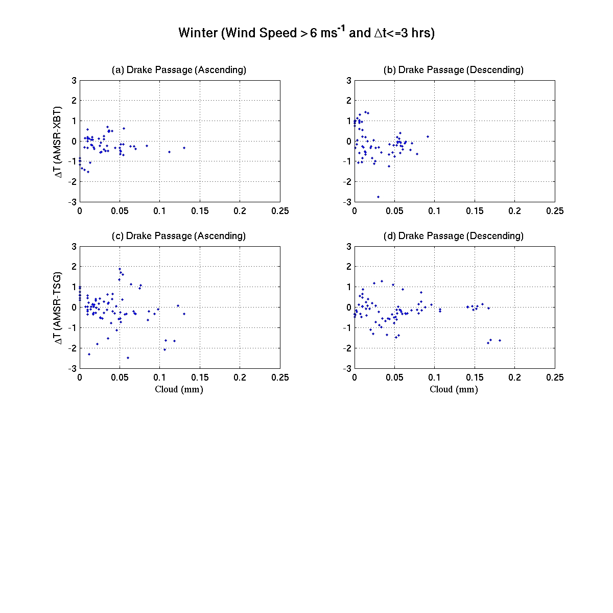
Temperature difference does not show close relationship with cloud ( Figure 10, Figure 11, Figure 12, and Figure 13).
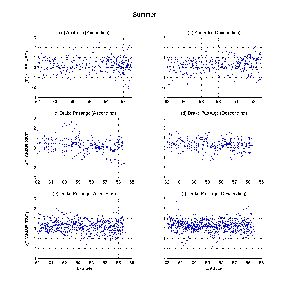
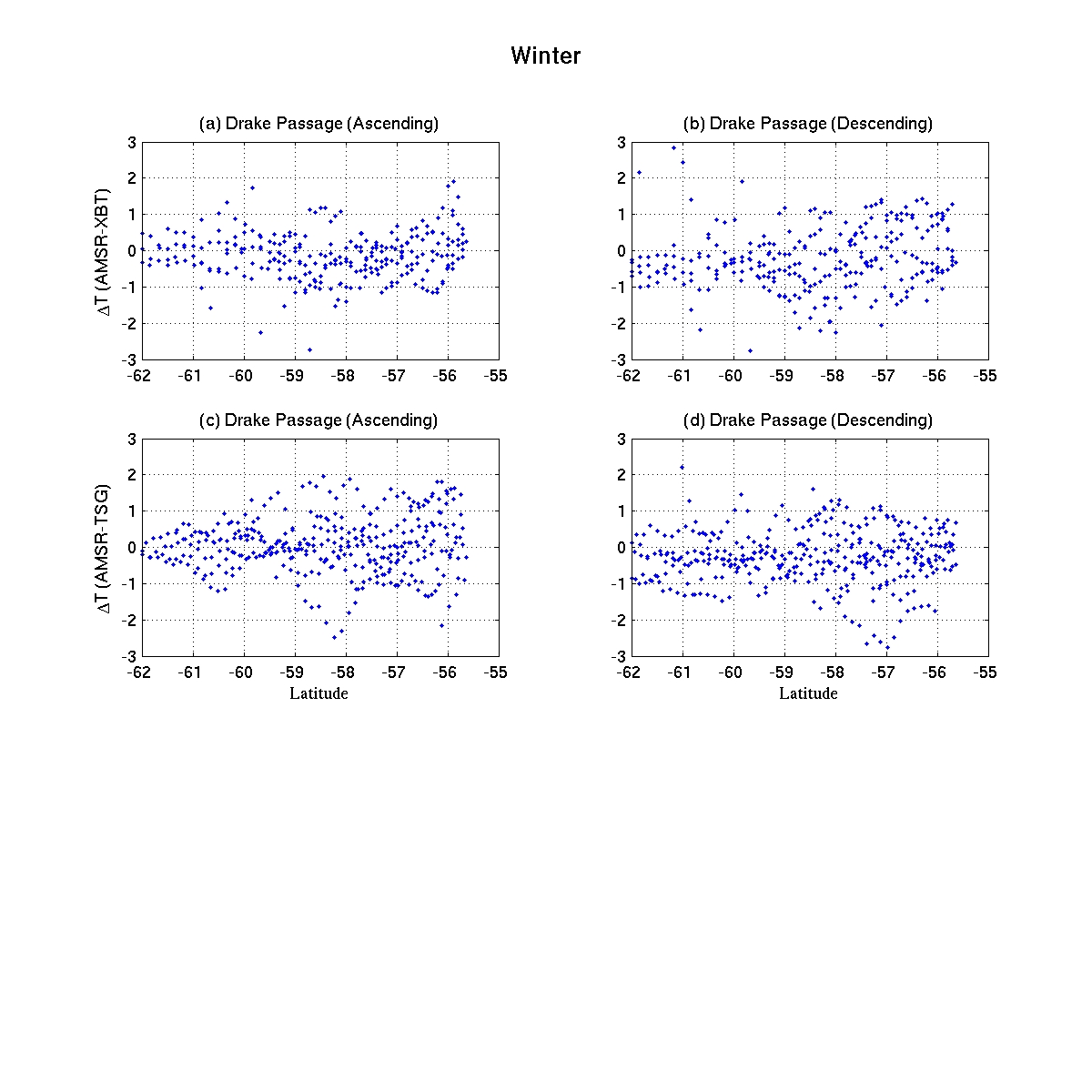
Temperature difference does not show close relationship with geographyic location (latitude) ( Figure 14, Figure 15, Figure 16, and Figure 17).
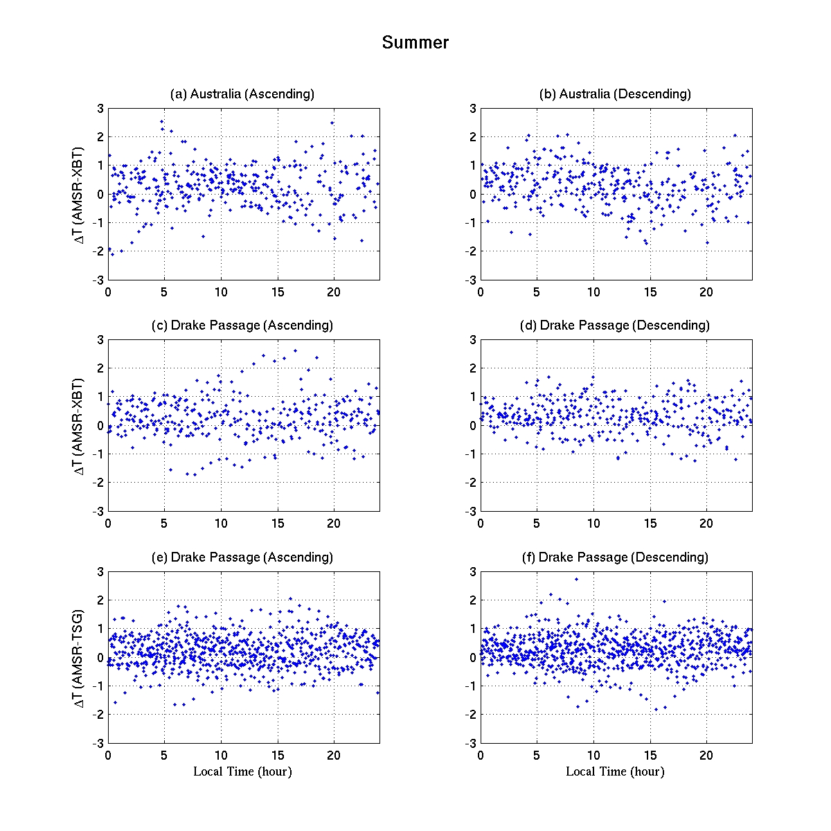
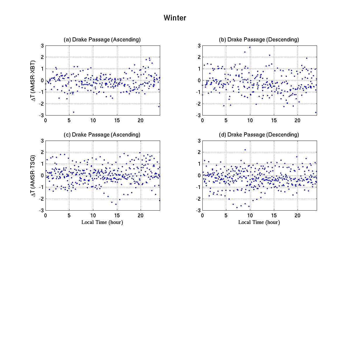
Temperature difference does not show close relationship with local time ( Figure 18, Figure 19, Figure 20, and Figure 21).
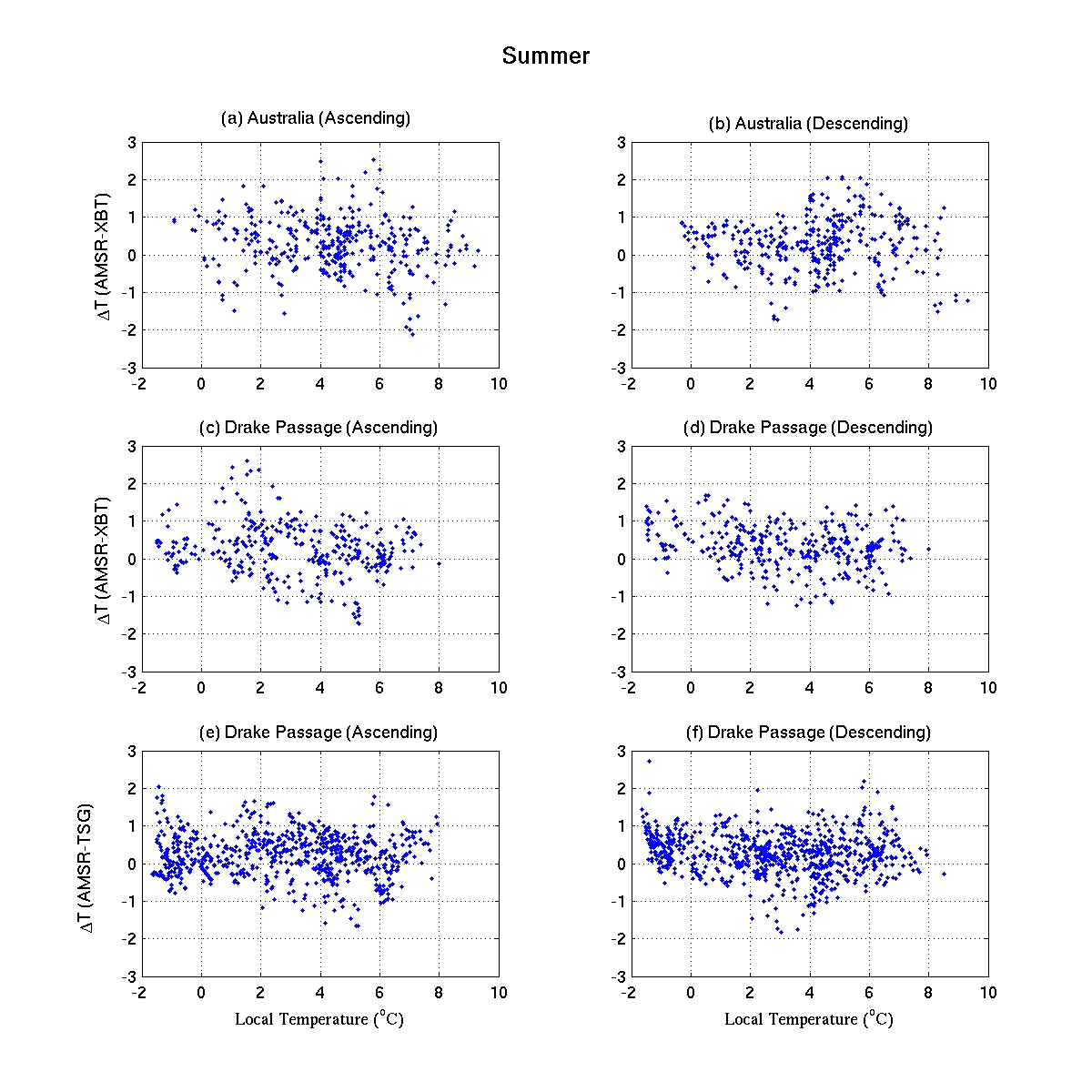
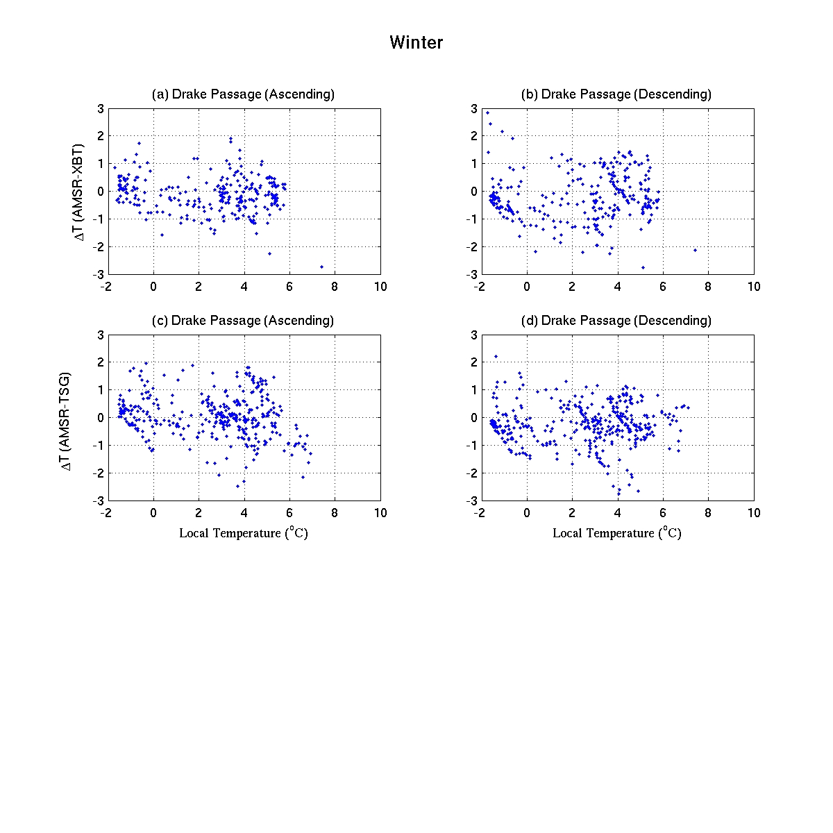
No apparent relationship between temperature difference and local temperature ( Figure 22, Figure 23, Figure 24, and Figure 25).
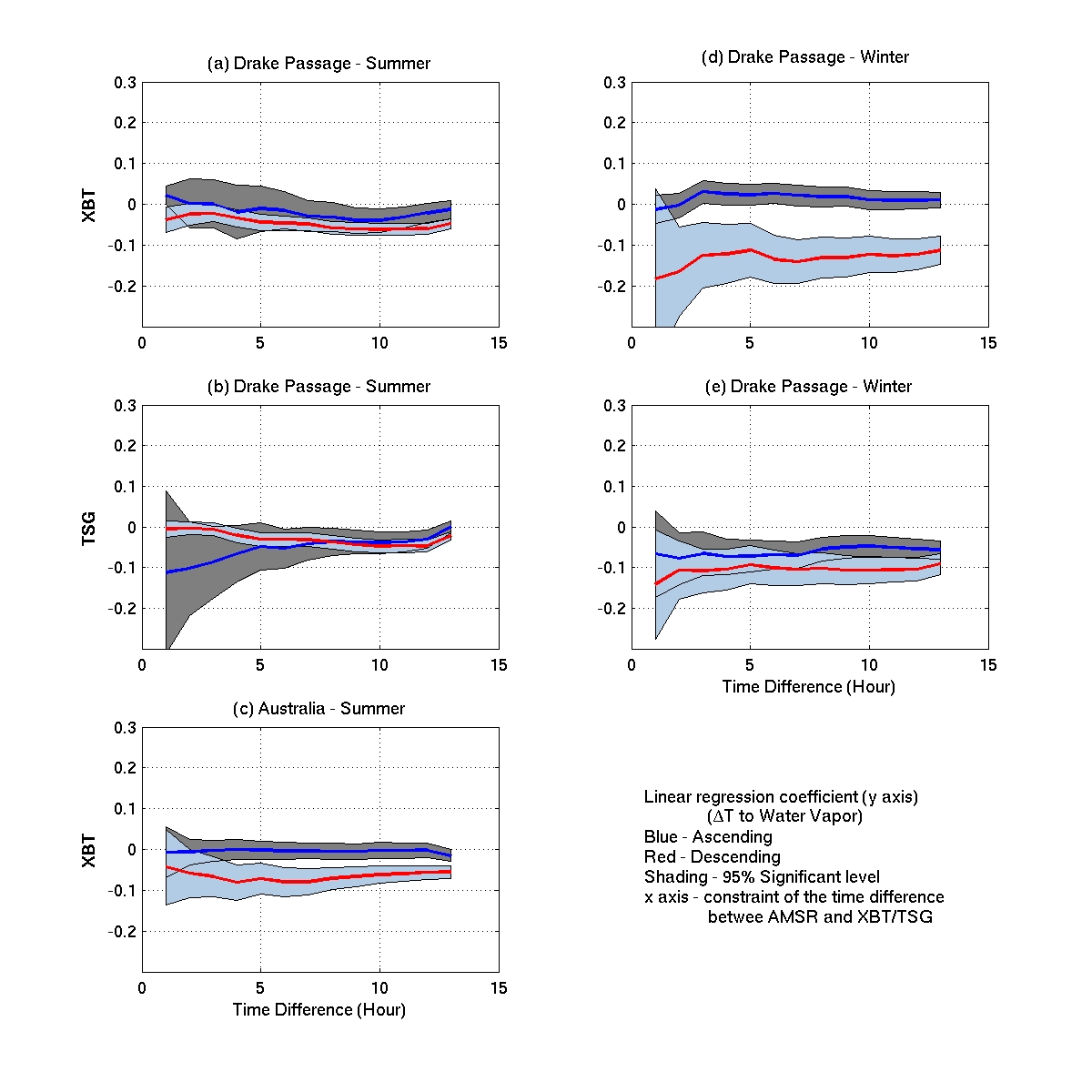
To summarize, the tempature difference is related to the wind speed (even without the low wind speed effect) and water vapor. This can also be seen from the linear regression. The following figures show the regression coefficient for wind speed and water vapor.
Figure 26 Scatter plots of the XBT/TSG against OI SST (interpolated into the XBT/TSG observation time and location). OI SST has warm bias.
Figure 27 Mean temperature difference between AMSR-E and OI SST.
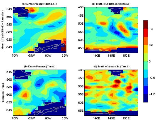
Figure 28 Example of SST from XBT, AMSR-E and OI.
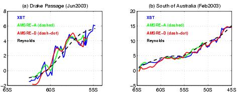
Figure 29 Scatter plots of the XBT against MODIS, (b) AMSR-E against MODIS, (c) and (d) temperature difference (AMSRE-MODIS) against wind speed and water vapor at the Drake Passage. The relationship between temperature difference and wind speed and water vapor are very similar to that for the AMSRE-XBT. For (b), (c), and (d) only the MODIS data within 1C difference from XBT is included. The cold MODIS is apparently cloud contamination. Also, low wind speed data is removed.
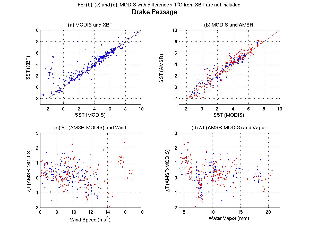
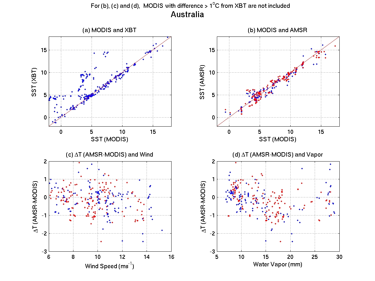
Figure 30 Same as Fig.29, but for south of Australia. I want to point out that, for south of Australia the mean difference between MODIS and XBT is not significant (0.04+/-0.03), but AMSRE is colder than MODIS (-0.16+/-0.07 (day), -0.18+/-0.06 (night)). At the Drake Passage, MODIS has a negative bias (MODIS-XBT, -0.1+/-0.02), and AMSRE is warm than MODIS (0.17+/-0.06 (day), 0.27+/-0.06 (night)).